3. Addressing Oversimplifications
Part II of this basic overview introduced some of the specialized vocabulary and graphical conventions used by chronobiologists. However, it included several simplifying assumptions regarding circadian clocks. A full understanding of circadian clocks requires seeing what these simplifying assumptions are, and seeing why they are oversimplifications. The task of this section is to address these points, by providing a fuller account of the complexities of Free-Running Periods (§3.1), and some more complicated details regarding entrainment (§3.2).
3.1. Variable FRPs: Aschoff’s Rules, Aftereffects & Temperature
In the foregoing we have often discussed free-running periods (FRPs) as if every member of the same species shares a single, fixed FRP. For example, we have said that the FRP for Mimosa plants is 22.5 hours. Likewise one sometimes hears that the endogenous free-running period of humans is about 24.2 hours. This is an oversimplification: the average FRP for a Mimosa plant lies somewhere between 22 and 23 hours, and the average FRP for humans comes out to about 24.2 hours. But there will be many individual differences between members of the same species.
FRPs can be even more variable than this: even for a single individual organism, the FRP can vary under varying environmental conditions. Among the first to study this phenomenon was Jürgen Aschoff, who established generalizations that later became known as Aschoff’s Rules. These rules work as generalizations for describing circadian phenomena and many organisms’ behavior; however they do not always hold true. (They are not exception-less laws). A review of FRPs, and an introduction to Achoff’s Rules, is available in the video below, called “Free-Running Periods."
Aschoff’s first rule is that the FRP of nocturnal organisms is typically less than 24. Aschoff’s second rule is that the FRP of diurnal organisms is typically greater than 24 hours. The third and fourth rules are our focus here: the FRP of an organism that is free-running in constant light (LL) will vary with changes in lighting intensity. The third rule is that increasing the intensity of light in LL will typically increase the length of a FRP in nocturnal organisms. The fourth rule is that increasing the intensity of light in LL will typically decrease the FRP in diurnal organisms. Both cases provide illustrations of how FRP is not constant, even within a single organism.
In addition to effects of age and lighting-intensity, there is another important way in which FRPs can vary. An aftereffect refers to lingering alterations of the clock induced by earlier environmental conditions. When an organism has been recently entrained and is then put into constant conditions, it will free run. However, how the organism had previously been entrained can have an effect on the FRP it now shows. An example is shown in Fig.3.1 below. Aftereffects show that zeitgebers leave thumbprints on circadian clocks, though such thumbprints may be erased in due time, or they may be counteracted through repeated exposure to new zeitgebers.
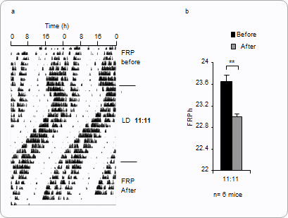
Figure 3.1:
a) The double-plotted actogram shows 48 hours of data on each line. The mouse is initially free-running. It is then entrained to an unnatural LD11:11 schedule. (Although the onset of activity is earlier each day, and the pattern of activity "drifts" to the left, this is not free-running: the mouse is entrained to 22-hour day, but the actogram still shows 48 hours of data on each line). After entrainment, the LD cycle is removed, and the mouse free-runs again.
b) Evidence of aftereffects in 6 mice that were put through this experiment. The FRP is significantly shortened after entrainment to the LD11:11 cycle. With time, the FRP would return to its earlier length.
Adapted by permission from Macmillan Publishers Ltd:
Nature Neuroscience (Azzi et al), copyright (2014)
Temperature can also affect FRPs, but the relationship between the clock and temperature is complicated. One of the defining features of a circadian clock is that it is temperature compensated. What this means, and why it is important, can be illustrated roughly through basic biochemistry. Most chemical reactions are highly sensitive to temperature, and occur at an increased rate if the temperature is increased. Circadian clocks in organisms depend upon biochemical processes to “tick” off regular increments of time. It wouldn’t make much evolutionary sense for an organism to develop a biological clock that was overly sensitive to temperature. For example, environmental temperature is very different in summer and winter, but the length of a day is always 24 hours. If the clock weren’t somewhat insulated from changes in temperature, it would “tick” at different rates throughout the year – which wouldn’t make it a very reliable clock at all. So it makes sense that circadian clocks should be temperature-compensated. An individual organism’s FRP stays relatively constant so long as it is in its physiologically and evolutionarily relevant environmental temperature range, regardless of whether the environment is cold (in winter) or hot (in summer). Despite this, there is individual variation in FRP, and likely individual variation in how well organism’s clocks are temperature compensated.
Box 3: A More Quantitative Introduction to Temperature Compensation
We can define temperature compensation more precisely (following Erwin Bünning, 1964) using a measure called the Q10 temperature coefficient.
Defining Q10
Q10 is a measure that can be applied the rates of both organic and non-organic chemical processes. Q10 is defined as a quantitative change in the rate of some process that is observed after increasing the temperature by 10°C. The precise formula is shown below:
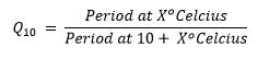
For most chemical and many biochemical reactions, it turns out that Q10=2 (or even 3). What this means is that increasing the temperature by 10°C tends to (roughly) double the rate of the reaction, so that it only takes half as long for the reaction to be completed. If, for some process, Q10=1, this would mean that the process is completely insulated from the temperature change, and its rate neither increases nor decreases by raising the temperature 10°C.
Q10 in Circadian Biology
In circadian biology, we are interested in understanding the biological processes which "tick" off time and give rise to an organism's free-running period (FRP). If those processes' rates were to increase with temperature, then the clock would run fast, and it would take less time to "tick." We would then expect the FRP to decrease as temperature increases. But in fact, organisms' FRPs tend to have a Q10 which is close to (but not exactly) 1: FRPs change comparatively little with changes in temperature. This is illustrated in the figure below. The blue line plots how much an FRP would vary with increasing temperature if it had a Q10=1.1 The red line plots how much an FRP would vary with increasing temperature if it had a Q10=2.0. The data one would observe for most circadian rhythms looks more like the blue line than the red line.
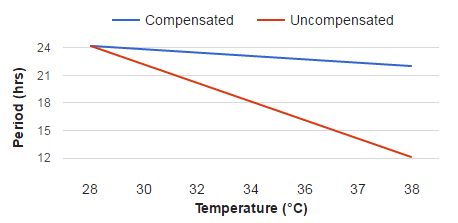
To say that for circadian rhythms, Q10≅1 is more precise way of expressing that the clock is temperature compensated.
Although circadian clocks are temperature compensated, acute changes in environmental temperature can in fact function as zeitgebers, and many organisms’ clocks can be entrained to a regular temperature cycle, or to a repeated increase or decrease of temperature. This is especially true for organisms that do not regulate their own body temperature. In organisms (like mammals) which do regulate body temperature, changing environmental temperature has less of an effect. For most organisms, light is by far a stronger zeitgeber than temperature. However, because temperature can have an effect on the clock, one can expect some individual variation in FRPs (even in organisms of the same species) if they are subjected to different temperatures.
To sum up this section: it is an oversimplificaiton to think that all organisms of the same species have precisely the same FRP, since factors like lighting intensity, aftereffects, and temperature can all produce individual variations.
3.2. Criteria for Entrainment, Skeleton Photoperiods, and Phase Response Curves
It is important to understand that entrainment – the synchronization of the clock to the environmental conditions – involves an effect of the zeitgeber on the actual “gears” of the biological clock; that is, a change in the internal, molecular mechanisms that regulate an organism’s activities. Masking (see §2.2 in Part II) must be carefully distinguished from genuine entrainment. There are four established criteria for determining when an organism is entrained to a cue. We have touched upon each of them above, but will now state them more clearly. A review of all four criteria is also available in the video below, called “Properties of Entrainable Oscillators."
First, in order to claim that an organism is entrained to a specific zeitgeber schedule, there must be no other time cues present to the organism. For example, if one wants to show that plants entrain to light-dark cycles, then one must control for temperature cycles: if one subjected the plant simultaneously to synchronized temperature and light cycles, then even if the plant entrained, there would be no way to confirm that the plant was entrained to light, and not to temperature. There would be no strong support for claiming that light was acting as the zeitgeber.
Second, whenever a zeitgeber is present, the organism must synchronize its rhythms, so that their period matches the zeitgeber’s period. (This is sometimes called the requirement of period control by the zeitgeber). For example, if an experimenter imposes a zeitgeber with the (artificial) periodicity of 24.3 hours (a “long day” that would not naturally occur), a mouse ought to be able to entrain to that cycle. If the zeitgeber is actually effective, we would expect the mouse’s onset of activity to occur once every 24.3 hours. In most cases, the requirement for period control is evident by adjusting the FRP to match a normal 24h zeitgeber.
Third, an effective zeitgeber must be shown to have its synchronizing effect reliably. For example, if we take the same organism and again subject it to the same zeitgeber schedule, then the organism ought to entrain to it again, with the same relative timing to the zeitgeber cycle. We should see again (for example) that onset of activity occurs once every 24.3 hours, and (if it is a nocturnal organism like a mouse) the onset of activity should occur at the start of the night phase. (This is called the requirement of a stable and repeatable phase relationship between the zeitgeber and the endogenous rhythm).
Fourth, if an organism is genuinely entrained to a zeitgeber, then when we remove the zeitgeber, two things should happen. First, the organism ought to begin to free-run, since the entraining and synchronizing cues are no longer present. Second, if the "gears" of the clock have actually been affected by the prior entrainment, then the organism should begin to free-run in a way that is determined by, and predictable from, its previous entrainment. (This is called the requirement of phase control.) This is what enables us to rule out mere masking as an alternative explanation for (merely apparent) entrainment in which only the “hands” of the clock are affected.
All four requirements are illustrated schematically in figure 3.2 below.
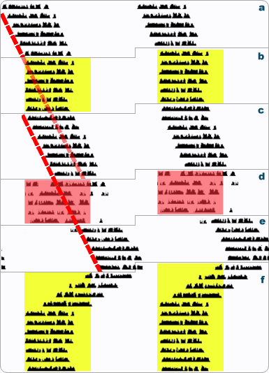
Figure 3.2 Criteria for Entrainment.
(a) A diurnal organism is free-running with a characteristically long (>24h) period in constant darkness, and all other zeitgebers that can be controlled are constant.
(b) The organism quickly entrains to an imposed LD12:12 cycle. Yellow shading indicates the light phase. (One sometimes needs to read captions: the conventional black and white bars are not always shown to indicate LD cycles). Since other zeitgebers have been removed (see a above), this is partial evidence that a light-dark cycle is an effective zeitgeber. The organism synchronizes to the LD cycle as evident by activity onsets aligning vertically. Thus, the period of the activity rhythm matches the period of the zeitgeber (24h) meeting the condition of period control.
(c) The LD cycle is removed, and the organism again free-runs. The FRP is >24h as before, but the onset of activity is predictable based on the prior, entrained phase of activity in b. Note the red line through successive onsets in part a does not align with the similar line for part c. Thus, entrainment in b exerted control over the clock's phasing to produce a several hour offset in the intervals of free-running, demonstrating phase control by light.
(d) A HotCold12:12 temperature cycle is imposed to mimic the prior LD cycle (red shading indicates time of high temperatures). During the HotCold cycle, the organism is in constant darkness so that light and temperature effects can be examined separately. At first glance, it appears that activity synchronizes to the temperature cycle. To see if this is really entrainment, however, again we must remove the putative zeitgeber (temperature) to see what happens.
(e) The temperature cycle is removed, and the organism free-runs. Note that the onset of activity is not predictable from the prior onset of activity during the temperature cycle in d: there is no evidence of phase control by temperature. Instead, comparing c to e by following the red line, the organism's clock has been free-running throughout d: the merely apparent synchronization to the temperature cycle was simply a form of masking.
(f) The LD cycle is imposed again, and the organism rapidly entrains again, demonstrating a stable and repetable phase relationship.
Thus far, we have discussed entrainment to LD cycles in which light is present throughout a long duration. In an LD12:12 cycle, the organism receives 12 whole hours of light. But notice that the four criteria for entrainment do not require that the zeitgeber resemble a natural day in this way (just as a zeitgeber does not have to have T=24h). A regular schedule of short pulses of light can also meet the criteria for entrainment. In extremely light-sensitive organisms, it has been shown that a regular daily pulse of light of only 1 sec in duration is sufficient to maintain entrainment. In many organisms, entrainment can be maintained with a daily light pulse of 15 - 60 minutes duration. For reasons that will become apparent later, investigators will sometimes investigate entrainment under skeleton photoperiods in which two light pulses are given daily. Instead of a full 12h light phase, for example, an investigator might replace 12h of light with two 1 hour pulses: one at the beginning and one at the end of the 12 h period. Under such conditions, entrainment is very similar to that seen with the a 12h photoperiod. This indicates that light at dawn and dusk (beginning and end of day) is doing most of the work of entrainment. An example is shown in Fig. 3.3 below.
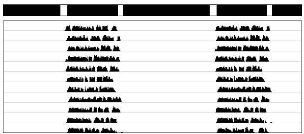
Figure 3.3: A double-plotted actogram, showing an organism entrained to a skeleton photoperiod.
Black and white bars at the top indicate when lights are on and off.
In both LD cycles and skeleton photoperiods, the organism is exposed to the periodic influence of some zeitgeber. But skeleton photoperiods show that isolated pulses of light can be effective in influencing and entraining the clock. A corollary of this is that entrainment may be study-able under highly simplified conditions whereby we investigate what happens to an organism when it is subjected only to a very brief and non-repeating light pulse (instead of a full 1 h photophase that repeats every 24h, as in the skeleton photoperiod above). Scientists are always looking to find the simplest conditions that elicit a particular effect because this allows all extraneous influences to be excluded.
In the case of circadian entrainment, application of brief (or "acute") light pulses to organisms reveals a fascinating and fundamental property of circadian clocks: brief light pulses cause circadian clocks to be reset, and the timing of the light pulse determines whether the light pulse will cause the resetting to be earlier, later or have no effect. In other words, there is a circadian rhythm in the response to a light pulse. Put another way, the effect that an isolated zeitgeber has on the clock depends upon the circadian time (CT) at which it is administered. Moreover, there is an adaptive logic to this rhythm: over evolutionary time, if there was a bright light in the environment it almost certainly came from the sun (lightning might be one possible exception). If an organism’s internal sense of time predicted that it was daytime, then experiencing bright light does not indicate that anything is counter to expectation. However, if the internal sense of time predicted that it was nighttime, the presence of sunlight indicates a mismatch with the environment that should be corrected. In the course of our evolution, the internal clock was less infallible than the rhythm of sunlight. Thus, our clocks evolved to reset themselves whenever their predictions of the current time of day were of sync with the lighting environment. With this evolutionary perspective in mind, we can begin to understand an important data graphic called a phase response curve.
Skeleton photoperiods show that brief light pulses are sufficient to support entrainment. An evolutaionary perspective enables us to conceptually understand why entrainment can occur in response to acute light pulses. If the clock of an organism currently predicts that it is day and the organism then experiences a bright light pulse, there is no indication that anything is amiss. The clock has no reason to make a correction. Empirically, across a vast array of species, a pulse of light in the subjective day has minimal effects on the circadian clock. Now suppose that a nocturnal rat wakes up to begin its nighttime activities. What does a bright light in the sky indicate to that rodent, when the organism is anticipating subjective night? Probably that it arose too early, because that bright light is probably the sun, which has not yet set. As a corrective, the rat might wish to make an adjustment to its internal sense of time and reset the clock so that the next day it gets up a little bit later. This kind of adjustment to the clock is called a phase delay. Conversely, consider a rat that has woken up and has been pursuing its activities in darkness for several hours. Everything seems in order: the rat anticipates subjective night, and the enfironment is dark. Suppose after several hours of activity, the rat’s internal sense of time indicates that it has 2 more hours of darkness to continue its nighttime activities. But if at this time, there is exposure to a bright light, the circadian system will interpret this as a sunrise. Clearly, the circadian system is running late and should have started and finished activity early than it did. Remarkably, a bright light pulse late in the subjective night causes organisms to reset their clocks so that their active phase begins earlier in the next cycle. This adjustment to the clock is called a phase advance. As these examples indicate, under natural conditions, small adjustments to the clock are usually made around dawn and dusk as clocks may deviate slightly from the proper phase. Organisms would rarely experience conditions where the clock became multiple hours out of alignment with the day-night cycle. Thus, what happens in response to light in the middle of the subjective night is not of great relevance to natural entrainment.
By graphing how much the circadian clock shifts in response to an acute zeitgeber, depending on the circadian time of the organism, we can produce what are called phase response curves (PRCs). A schematic example is shown below. The X axis tracks the time at which a zeitgeber is applied, and on the Y axis, we plot how much it affected the clock.
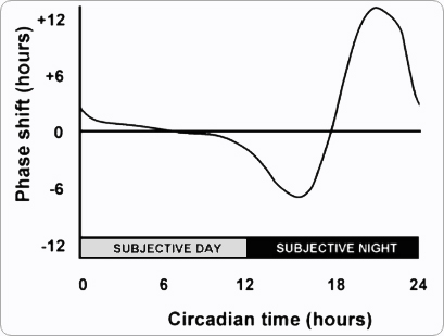
Figure 3.4: The basic shape of a PRC.
A phase response curve (PRC) can summarize a tremendous amount of data regarding how a zeitgeber affects an organism’s clock. Two videos, embedded below, explain how PRCs are constructed. First, a video on “Naming Conventions” explains the terminology of “phase shifts.” Second, a video on “Phase Response Curves” explains how a PRC summarizes data about phase shifts in response to a zeitgeber. We will briefly review the basics below, using an example in which light is used as a zeitgeber.
To gather the data for a PRC, scientists experiment with variations on light-dark cycles by using acute light pulses, during which the lights go on for a predetermined period of time before going out. For example, a light pulse might be fifteen minutes long, much less than the light duration of light in a natural daily cycle. These light pulses cause phase shifts, or changes in the timing of the onset, offset, peak, or other notable feature of a circadian rhythm. For example, an acute light pulse to a free-running rat might alter when its next onset of activity occurs.
A PRC relies on the fact that phase shifts can be precisely quantified. By convention, phase shifts are distinguished as positive or negative. A negative phase shift signifies a delay. For example, suppose a rat is free-running, and its onset of activity is occuring with a short period, once every 23.5h. We now apply an acute light pulse, and we find that after the pulse, the next onset of activity occurs 23.9h after the previous onset of activity. The onset of activity was delayed by 0.4h compared to when we would have predicted its occurence on the basis of FRP. We would say that the light pulse caused a negative phase shift of 0.4h. Conversely, a positive phase shift indicates an advance. Suppose a light pulse caused the rat's next onset of activity to occur 23h after its previous onset of activity. The onset of activity was advanced by 0.4h. We would say the light pulse caused a positive phase shift of 0.4h.
What we have illustrated in these brief examples is that whether a light pulse causes a positive or a negative phase shift depends on when the pulse is delivered with respect to the organism’s circadian time. An pulse of light during the organism's subjective day will have a different effect than an identical pulse of light during the organism's subjective night. In our example above, it could have been the very same light pulse (the same duration, the same light intensity, etc.) that caused a positive phase shift or a negative phase shift of 0.4h: the organism's response depends on the phase of circadian time in when the pulse is applied. The phase response curve provides a quantitative representation of this phenomenon, plotting phase shifts as a function of circadian time.
With the way that an organism's clock and its PRC is built, an organism is always able to change its internal clock to fix itself when put in a periodically light and dark environment. The "dead zone" is the organism's "sweet spot," and the clock will reset itself so that the dead zone aligns with the middle of the light phase. If light ever occurs with too much deviation from the sweet spot, the PRC shows us how the organism's clock will phase shift positively or negatively until the "dead zone" matches mid-day.